The floating-point trick is more surprising
A naive design might subtract the previous floating-point value from the next one, then store the numerical difference. But approximate numeric similarity is not always the same as similarity of IEEE 754 bit patterns, and subtraction introduces its own representation concerns.
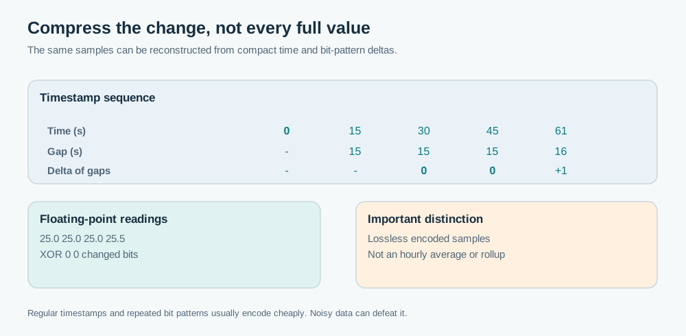
The Gorilla-style approach instead compares the 64-bit encodings of consecutive floating-point values using XOR. If two values are bit-for-bit equal, the XOR result is zero. That can be represented very cheaply. If only a few bits changed, the XOR may contain long runs of leading or trailing zeros. The encoder can describe a significant-bit window and store only the bits needed for the change.
Take the readings 25.0, 25.0, 25.0, 25.5. The first value establishes a full representation. The two repeated readings have zero XOR. The final change alters the bit pattern, so it requires additional information, but still may be cheaper than another full 64-bit value. If values jump unpredictably or contain noisy low-order bits, the advantage becomes smaller.
The important word is lossless. XOR encoding lets the decoder reconstruct the exact stored floating-point bit patterns under that encoding's supported semantics. It is not rounding sensor readings or estimating missing observations. This is different from downsampling, which deliberately reduces time resolution and cannot usually recover every original sample.
The original Gorilla paper describes delta-of-delta timestamps and XOR floating-point values as key ingredients in a monitoring-oriented TSDB. Prometheus's published chunk format also documents these techniques in its XOR chunks. These are concrete implementations, not a guarantee that all TSDBs use an identical bitstream. Gorilla, VLDB 2015 and Prometheus chunk format.
Compute the upper bound before claiming a win
Ten million observations represented as a raw pair of two eight-byte values require 160 million bytes of sample payload, which is about 153 MiB. That calculation ignores metric labels, series metadata, indexes, chunk headers, storage replication and WAL overhead. It is a baseline for the two fields, not a prediction of total TSDB disk usage.
Suppose most timestamps follow a 15-second interval and most sensor values either repeat or change slightly. Many later observations can fit into far fewer than 128 bits. In a different workload, each reading may use a new random timestamp interval and a noisy float. The same algorithm can then spend much more space per observation.
Also notice that compressing a series well does not make a million one-sample series cheap. Each isolated series still needs identifying metadata, and it has little history from which to learn repeated timestamp gaps or value patterns. That connects to our previous episode about cardinality, but the core mechanism here is per-series compression.
Walk one sample through a real storage path
In a Prometheus-style design, a freshly ingested sample reaches an in-memory head structure and a write-ahead log for crash recovery. The compressed chunk representation and the on-disk block index are not simply one big ZIP file. Recent WAL bytes can be much larger than compacted chunks. Block compaction may rearrange chunks and metadata later.
A query by metric labels first has to find the relevant series. The index tells the engine which series match. The engine then locates chunks for the time range and decodes their sample sequence. Compression helps with IO and memory bandwidth, but the index and the number of matching series can still dominate a query. This is why a TSDB needs both efficient data encoding and efficient access paths.
There is also an ingestion-time complication: out-of-order timestamps. A decoder optimized for monotonic timestamps and nearby samples does not necessarily accept arbitrary late samples into an existing compressed sequence. Different engines buffer, reject, rewrite or use separate backfill mechanisms. It is unsafe to infer supported late-arrival behavior from the compression algorithm alone.
What I would optimize next
If the business needs an exact audit of every sensor reading, preserve raw points for the required period. If it needs only monthly trends, retention and rollups may save more query work than another encoding tweak. Those are separate decisions with separate correctness costs.
I would benchmark compression using realistic sensor distributions, timestamp jitter, counter resets, special floating-point values and series churn. Measure end-to-end ingestion CPU, query decode cost, index and WAL sizes, not only bytes per compressed sample. A Staff-level answer should be able to explain why the bits are small and why that does not automatically make the entire storage service cheap.