Interview question. A shared dependency handles about 850 operations per second and is already busy. Incoming traffic increases by 15 percent. The query code, database indexes, and average cost of individual operations do not change, but response time becomes far worse. Explain the relationship between utilization and waiting time. What would you measure before buying more hardware?
Do not assume a universal CPU threshold at which every system collapses. We will first use a simple queueing model to understand the shape of the problem, then return to real systems where service times and arrivals vary.
Think first
A storage service can complete about 500 small operations per second on one saturated bottleneck. Arrival rate moves from 450 to 495 per second. Use a stated model to estimate the delay change, then explain why your estimate might be wrong for production.
Take a few minutes to form an approach, then compare it with the worked explanation.
Check the exercise numbers
Under the stated M/M/1 assumptions, W = 1 / (500 − 450) = 20 ms, then W = 1 / (500 − 495) = 200 ms: a tenfold increase in model mean response time. These are not production p99 predictions. With three equal zones, surviving one loss leaves two-thirds of total safe capacity before burst and repair allowances.
Reveal the worked explanation
Work can arrive faster than free capacity appears
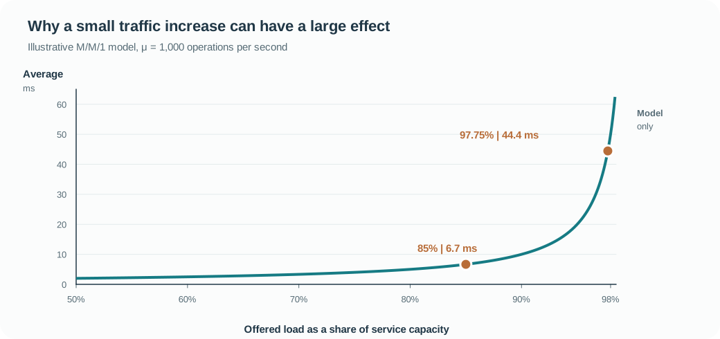
Imagine a single service station that can complete an average of 1,000 operations per second when continuously busy. At 850 arrivals per second it has some room for bursts and variation. Increase arrivals by 15 percent and the rate becomes 977.5 per second. The station has not hit its nominal limit, but the room for clearing a queue has shrunk sharply.
For a textbook M/M/1 model, with random independent arrivals, exponentially distributed service times, one server, and stable utilization, average time in the system is:
W = 1 / (μ - λ)
Here μ is the service rate and λ is the arrival rate. We can calculate the change:
Before: μ = 1,000/s, λ = 850/s
Average response time = 1 / (1,000 - 850) = 6.7 ms

After:  μ = 1,000/s, λ = 977.5/s
Average response time = 1 / (1,000 - 977.5) = 44.4 ms

Traffic increases 15 percent
Modeled average response time increases about 6.7 times
Those values are consequences of this illustrative model. They are not a measured database benchmark, nor do they imply that every system follows the same curve. The important discovery is the shrinking difference between how fast work arrives and how fast it can leave.
Queueing model showing rapidly increasing response time as utilization approaches the service limit
Real traffic makes the tail less friendly
Production arrival patterns are not necessarily memoryless. A marketing campaign sends correlated bursts. One customer can issue unusually expensive queries. Background compaction may steal disk bandwidth. A query plan can change as a result of different parameter values. So average arrival rate alone does not capture the queue's behavior.
Variance matters because a long operation keeps the shared station occupied while other work accumulates. Two workloads with the same average query execution time can have very different p99 latency if one contains occasional expensive operations.
For that reason, I would not conclude “the database is 98 percent utilized, so add replicas” from a CPU dashboard alone. Which resource is busy? Is it CPU execution, disk I/O, a row lock, an internal thread pool, a storage device queue, or an external service? If the database is blocked on one hot lock, ten more CPU cores may do nothing. A measured 98 percent CPU can also conceal different demand patterns from a measured 98 percent disk saturation.
The first useful plot is arrival rate, completion rate, queue depth or oldest waiting age, and request duration over the same interval. As the queue starts to grow, the service may still look productive because completions continue. The warning is that arrivals consistently exceed completions or that the capacity margin has become too small for normal bursts.
Protect tail latency by reserving room for uncertainty
Headroom is not simply idle hardware that finance wants to reclaim. Its purpose is to absorb variation, repair work, zone loss, deployments, and short bursts without turning them into enormous queues.
How much headroom is enough depends on workload shape and the failure model. If a service spans three equal-capacity zones and must survive losing one, a design that requires more than the remaining two zones' safe capacity cannot meet that failure objective without shedding traffic or degrading work. Add burst demand and repair cost to the same calculation. A 70 percent utilization target might be too high for one service and unnecessarily conservative for another.
There are several different interventions, and I would not apply all of them reflexively. If a small set of queries are unusually expensive, isolate or optimize them. If requests perform unnecessary serial work, reduce the critical path. If the service truly needs more capacity, scale the saturated resource and verify that the next bottleneck has not merely moved. If demand exceeds acceptable latency even with scaling, use admission limits and clear rejection rather than allowing an enormous queue to form.
Queueing for a short burst can be reasonable when the caller is willing to wait and the backlog will clear before its deadline. An unbounded waiting room is not a reliability mechanism. Google SRE's discussion of cascading failures makes the same practical point: queue growth consumes resources and can worsen a struggling service's recovery. [1]
I would not reduce this to “latency explodes at 90 percent.” It is memorable but technically misleading. Show the model’s assumptions, calculate the shrinking capacity margin, and investigate the actual limiting resource.
Now add one more complication. A call waits so long that its client retries. That second attempt enters the same saturated system while the first may still be running.
Can the recovery mechanism itself become the source of the outage?
Go deeper
What the curve leaves out
The M/M/1 model assumes one server with independent Poisson arrivals and exponential service times. The formula W = 1 / (μ - λ) gives the model's mean time in the system, including service. It is not a formula for every real p99. Real services have parallel workers, changing workloads, priorities, finite buffers, client cancellations, and resources that saturate at different rates.
In the same model, utilization is ρ = λ / μ, so a 15 percent arrival-rate increase from 850 to 977.5 per second moves offered load from 85 percent to 97.75 percent. The available completion-rate margin shrinks from 150 to 22.5 per second. That approximately 6.7-fold reduction in margin is why small fluctuations become costly near saturation.
Measure service-time distribution as well as its average. If one database transaction sometimes holds a lock for 100 ms while most use it for 1 ms, the queue can suffer without a change in mean request size. Choose an analytical model only after observing whether its assumptions roughly fit.
The same failure-headroom calculation should be made with safe sustainable capacity, not a benchmark obtained while ignoring p99 objectives. Surviving one of three equal-capacity zones implies that the remaining zones must be able to serve the admitted load. Maintenance, repair traffic, and the risk that failures are correlated also matter.
Check your reasoning
State a queueing model explicitly rather than making universal claims about percentages.
For M/M/1, calculate W: 20 ms at 450/s and 200 ms at 495/s.
Identify variance, correlated bursts, long operations, and finite queues as violations of simple assumptions.
Propose sufficient headroom, workload isolation, optimization, or admission based on diagnosis.
Common mistake: Treating “90 percent utilization is bad” as a law that gives a precise p99 for every storage system.
Read the answer explanation
No, it depends on restrictive assumptions and describes a model. — Use the model to explain why the margin shrinks. Real systems require measured service-time distributions, workload shape, and bottleneck analysis.
Apply it elsewhere
A database has normal average query time but large p99 spikes during compaction. Would adding CPU solve it?
Compare your approach
Do not guess. Identify whether compaction steals disk bandwidth or cache, examine queue age, and isolate or schedule the competing work based on the actual resource bottleneck.
One more constraint
A whole availability zone fails. How would you derive safe steady-state utilization for the surviving capacity?
Quick revision
Near saturation, a small increase in arrival rate leaves very little spare service capacity to clear bursts. Under an explicitly simplified M/M/1 model, a server with capacity 1,000 operations per second has mean response time about 6.7 ms at 850 arrivals per second and about 44.4 ms at 977.5 arrivals per second. That is roughly a 6.7-fold increase from 15 percent more traffic. I would not claim those are universal p99 results. Real systems have parallel workers, bursty arrivals and variable operation costs. I would measure actual queue depth, arrival and completion rates, time spent waiting, service-time distribution and saturated resources. The fix might be headroom, isolation, optimization, scaling or controlled admission, depending on evidence.