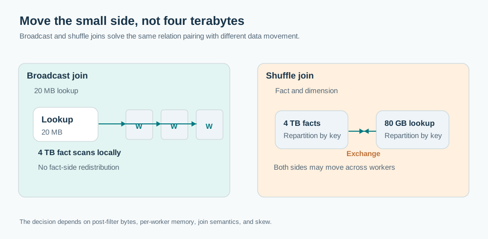
A team has a 4 TB fact table of product views and a 20 MB table mapping product IDs to categories. Both are stored in a data lake. A Spark SQL query joins them to count views by category. The query scans the large fact table and then triggers a huge network shuffle.
Interview question. Choose a distributed join strategy, estimate its data movement and memory costs, and explain why a query planner could make a worse choice than expected. Then change the small table into an 80 GB dimension and reconsider the plan.
This lesson is about where rows need to meet across machines. A local hash join builds a lookup structure and probes it on one worker. The distributed problem first decides which rows must reach that worker before it can match them.
Think first
A 6 TB table joins with a 40 MB filtered lookup. The query shuffles both sides and the lookup is unique by join key. Propose the plan, estimate the broadcast footprint across 60 workers, and list two reasons a broadcast still might fail.
Take a few minutes to form an approach, then compare it with the worked explanation.
Check the exercise numbers
For 60 workers, one 40 MB filtered lookup copy per worker is about 2,400 MB = 2.4 GB of aggregate payload before overhead. Each worker must still hold its decoded build-side representation alongside concurrent work. Broadcast can fail because that representation exceeds memory or because distribution exceeds the broadcast timeout; the 6 TB fact table still has to be scanned.
Reveal the worked explanation
The cheap option depends on which side moves
If the 20 MB product table fits comfortably in the usable memory budget of each worker, broadcast it to the workers already scanning the views. Each worker can join its local fact-table partitions against an in-memory copy of the product table. The 4 TB fact table does not need to be globally reshuffled just to find category labels.
Suppose the job has 80 workers and each gets one 20 MB copy. An illustrative total is about 1.6 GB of distributed payload, ignoring protocol overhead, retries and any repeated broadcasts. More importantly, per worker the build-side representation must fit with other operators and concurrent tasks. A 20 MB compressed file can occupy more memory after decoding and building a hash table.
The input still has to be scanned. Broadcasting does not make 4 TB vanish. It avoids redistributing that large fact side for this join. If the final aggregation groups by category, the partial counts may still need a smaller exchange later.
Apache Spark supports broadcast joins and several shuffle-based join strategies. A hint expresses a preference rather than a guarantee that a strategy is valid for every join type. The runtime plan, available statistics and size of the actual build side matter. Spark SQL performance tuning
Broadcasting a 20 MB lookup to workers avoids shuffling a large fact table, unlike a two-sided shuffle join.
Why did the engine shuffle four terabytes?
Start by reading the physical plan. Did the system choose a shuffle join because it thought the dimension table was much larger? Did the join happen before a selective filter? Was the small table padded into a wide intermediate relation containing columns not used by the query? Was broadcasting ruled out by the configured size threshold or join type? If an attempted broadcast ran out of memory or timed out, inspect the failure; do not assume Spark automatically retries every failed broadcast as a shuffle join.
The documented automatic broadcast threshold is 10 MiB by default in the linked Spark version, so a 20 MB lookup may already exceed it without any bad statistics. Check the actual configuration before blaming the planner. Statistics are especially important. A catalog might report that the dimension contains several billion rows from a previous version, while the filtered relation is actually tiny. Or a query might use a function on the join key, making partitioning information unusable. An optimizer could also make a reasonable choice based on an earlier stage whose cardinality estimates were wrong.
I would inspect estimated row counts alongside runtime row counts and sizes. Then I would check where projection and filters are applied. Removing twenty unnecessary columns before an exchange sometimes matters more than increasing network bandwidth.
If you must shuffle both sides, each input is repartitioned using a compatible function of the join key. Rows for one product ID are sent to a common destination. A worker can then join the two local partitions. That enables a distributed join but costs serialization, network transfer, potential spill, and possibly skew when some keys occur far more often than others.
A join can also have a severe skew problem even when the overall fact table is well distributed. If one product represents 30 percent of all views, all its rows may arrive at one join partition. A general increase in shuffle partitions does not change which partition owns that product key. The heavy-key alternatives now depend on whether the matching dimension row can be replicated and whether the join semantics allow a split.
Now the dimension grows to 80 GB
Broadcasting 80 GB to every worker would be a very different proposition. At 80 workers, the uncompressed aggregate payload is 6.4 TB before memory representation or network overhead. It may be impossible for an individual worker to hold the build side at all. Broadcasting is no longer the obvious choice.
A shuffle join may become appropriate. If both datasets are already partitioned on the same key with compatible conventions and trustworthy layout, some exchanges can be avoided. If a filtered subset of the 80 GB dimension is genuinely small, broadcasting that subset might still work. There is no timeless rule that says dimension tables always broadcast.
A physical plan should be justified with the actual post-filter sizes and memory per executor. Pinning a BROADCAST hint without checking those facts can convert a network problem into out-of-memory failures.
An interview answer should include the output contract
Suppose the dimension has two category rows for the same product ID. Joining can now duplicate a fact row even if the distributed strategy is otherwise correct. A faster join would simply produce a wrong count faster. Before measuring performance, confirm whether this is a one-to-one lookup, a versioned mapping, or intentionally one-to-many data.
For a versioned product catalog, an event-time category might be required rather than today's category. That affects the join condition and the data that must be retained. It is a business correctness question, not a shuffle optimization.
If I could ask the interviewer only one clarifying question, it would be: After all filters and projections, how large is the unique lookup relation per worker? That answer drives the next design decision far more directly than the raw size printed on the source table.
The team adopts the better join strategy and the daily job becomes fast. But analytics queries are still slow after the output reaches object storage. Our next problem is why the same bytes behave differently when broken into thousands of tiny files.
Go deeper
Optional depth: broadcast and planner adaptation
Broadcast distribution and join-local hash tables are separate costs. Broadcast may require transferring and caching the relation per executor, while concurrent tasks may each have their own execution structures. Spark Adaptive Query Execution can sometimes change the join strategy using runtime statistics after a shuffle boundary, but it cannot always eliminate work already paid to produce that shuffle. Inspect the executed plan rather than assuming the optimizer removed every unnecessary exchange.
Check your reasoning
Broadcast the small relation when its memory footprint is safe.
Estimate replicated bytes and per-executor memory, not only source table size.
Distinguish a scan of fact data from redistributing fact data.
Handle larger build relations, join skew and duplicate lookup keys.
Common mistake: A broadcast join means no scan or communication remains.
Read the answer explanation
Broadcast a safe lookup copy and scan fact partitions locally — A small broadcast side can avoid repartitioning the fact relation.
Apply it elsewhere
A fraud system matches all transactions against a small high-risk merchant list that changes during a run. What consistency policy is needed?
Compare your approach
Decide whether the join uses one stable snapshot of the merchant list or allows updated versions mid-query.
One more constraint
Does broadcasting the lookup mean the query performs no network communication at all?
Quick revision
When one join side is truly small, broadcast it to the workers scanning the large side and join locally. That may avoid shuffling terabytes of facts, though scanning and final aggregation still cost resources. For large join sides, use compatible partitioning and a shuffle strategy. Confirm actual post-filter sizes, memory and output multiplicity before forcing a hint.