Interview question. Your team runs a nightly job over 10 TB of click events to calculate counts per campaign. Reading the files takes 14 minutes. The next stage transfers data between workers, spills to disk, and runs for more than an hour. Explain what actually moves during a shuffle, why adding more executors may not help, and what you would measure before changing the cluster.
Assume the input contains many events per campaign, counts are additive, and the output needs one total per campaign. There is no requirement to preserve individual event ordering.
Think first
The input reads 10 TB and the shuffle writes 7 TB. Sixty percent of the stage time is disk spill. Describe the first three measurements and the design changes you would try, in priority order.
Take a few minutes to form an approach, then compare it with the worked explanation.
Reveal the worked explanation
Follow one event to its destination
A file may be split into input ranges, and different workers can read those ranges at the same time. That makes scanning scalable. But a campaign's events are scattered across files, so the worker reading an event cannot necessarily finish that campaign's count on its own.
Suppose one worker sees three clicks for campaign C17 and another sees four. Someone has to combine them. The system needs a rule that sends the partial values for C17 to the same logical destination. This redistribution is the shuffle.
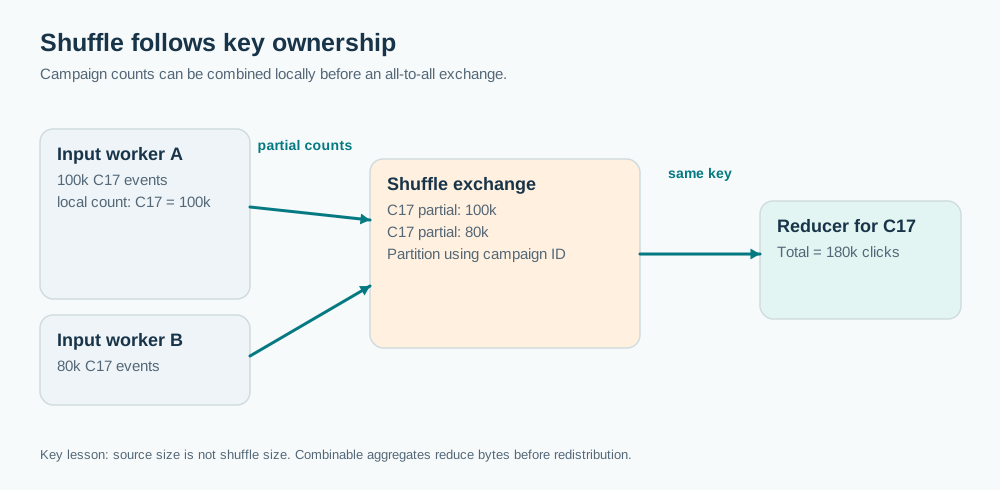
Input workers locally count campaign C17 events and send small partial counts across a shuffle to a reducer.
The names map and reduce describe roles, not necessarily one map task per file or one reducer per campaign. A map-side task produces intermediate records or partial aggregates. The shuffle groups them according to a partitioning rule. Reduce-side tasks receive the material they need and complete the computation. Spark uses shuffle boundaries for operations such as repartitioning, grouping, and joins. Its documentation explicitly describes network traffic, serialization, disk I/O, and spills as costs of this step. Spark RDD guide
So the first interview question I would ask is whether the job is moving the original click events or substantially smaller partial counts. Those are two very different architectures.
Do less work before moving anything
Because counts can be combined, each input task can aggregate locally. Instead of sending 100,000 copies of (C17, 1) from one task, it can send (C17, 100000). The destination adds the partials.
This is safe because addition is associative. For exact integers in a sufficiently large representation, regrouping the additions preserves the result. It is not automatically safe for an arbitrary function. Taking the average of two averages without their counts is wrong when group sizes differ. Sending only the latest event based on whichever row happened to arrive last is also not an order-independent reduction.
Consider a hypothetical 10 TB input with a billion records and a million intermediate partial groups after local aggregation. If each partial is 32 bytes, that material is roughly 32 MB before serialization overhead, not 10 TB. That enormous reduction is possible only when the grouping structure and workload really permit it. A campaign with one event per unique key would not shrink in the same way.
In a physical execution plan, look for partial aggregates before the exchange and a final aggregate after it. In an RDD program, distinguish reduceByKey from groupByKey when the goal is an associative reduction. They do not have identical intermediate data volumes. Spark RDD guide
Where did the hour go?
I would open the stage metrics, not increase the worker count immediately. How many shuffle bytes were written and fetched? Is the time spent waiting for remote blocks, sorting, spilling, garbage collection, or computing the reducer? Are a few reduce partitions dramatically larger than the median? Does the scheduler have pending tasks while some machines are idle?
Network bandwidth is only one possible limit. A reducer might spend most of its time sorting a large partition or repeatedly spilling it. The producer side might be writing shuffle files slowly because local disks are overloaded. Some blocks may need to be fetched again after an executor fails. More executors can add request concurrency without increasing the bandwidth or disk capacity of the machine holding the data.
There is another trap in the 10 TB figure: it is the input size, not a prediction of the shuffle size. A group-by with useful partial aggregation may shuffle far less. A join or expansion that multiplies records may shuffle more. You need measurements of the actual exchange rather than reasoning from input bytes alone.
When would you change the design?
If expensive data movement is unavoidable, I would first prune unused columns and rows before the exchange. If aggregation is possible, aggregate locally. If the data is already partitioned compatibly by campaign and its properties can be trusted, an extra exchange might be unnecessary. If partitions are uniformly too large, more suitably sized reduce partitions can increase parallelism, provided there are resources to run them.
But if one campaign dominates the data, a larger partition count does not automatically split that campaign. The partitioning function still sends its key to one destination. That is the problem in our next interview question.
Practice before continuing. A new team changes countByCampaign to calculate the exact median session length per campaign. Which optimization from this answer is no longer straightforward, and what state would you have to preserve to produce the exact result?
Go deeper
Optional depth: what shuffle files mean for recovery
A shuffle usually creates intermediate output that can be reused by downstream tasks, but it also introduces a recovery boundary. If a machine holding intermediate files disappears and no durable copy is available, upstream work may have to be recomputed. In a lineage-based engine that can be acceptable, but long input stages and expensive joins make replay costly. Look at where intermediate files are stored, which fetch failures trigger stage retries, and how aggressively the engine removes intermediate data. Be careful not to describe every Spark deployment as having the same shuffle-storage behavior, because external shuffle services and newer shuffle mechanisms change the details.
Check your reasoning
Identify grouping requirements and the all-to-all exchange.
Compare actual shuffle bytes with input bytes and stage-level spill metrics.
Move associative aggregation toward the scan and explain when it is unsafe.
Reject adding workers as a universal fix for one hot key.
Common mistake: More workers always reduce shuffle cost, regardless of partition size.
Read the answer explanation
Whether map-side partial counts would move fewer values — Counting can be partially aggregated, reducing the records moved across the exchange.
Apply it elsewhere
A log analytics job groups records by tenant and then computes an exact percentile. What changes?
Compare your approach
An exact percentile needs enough distributional information to merge partial states without changing the answer.
One more constraint
Would `groupByKey` followed by `size` generally be preferable to a combinable key count? Explain what travels over the network.
Quick revision
A shuffle redistributes records or partial aggregates so data for one key can be processed together. Its cost depends on bytes moved, partition skew, serialization, network fetches, local disk and spill, not just source size. I would inspect the exchange plan and per-task metrics, reduce data before the exchange, and size the partitions from the measured workload. If one key dominates, more partitions alone cannot fix it.